This is part of the Road/Transportation network at Gang (contact).
This fairly simple question raises a not-so-easy graph problem: computing the diameter. That is find a pair of points such that their distance is maximal. We call diameter path a shortest path between these two points. More precisely, the distance we consider here is the travel time. If you always follow the fastest path in your trips, then the diameter path of the world is the longest road trip you can plan.
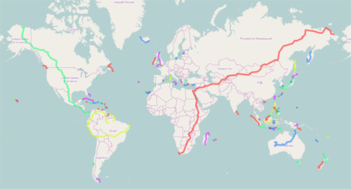
Click on the following map to zoom in the longest road trips of the largest components of the world road network.
The diameter path of the world road network (the red path in the above picture) appears to go from Capetown to Russian far east. Driving at speed limits, it is 10 days and 8 hours long. Its length is 25200 Kms (15700 miles). The trip must be done in winter as some parts appear to lie on rivers towards the end of the path.
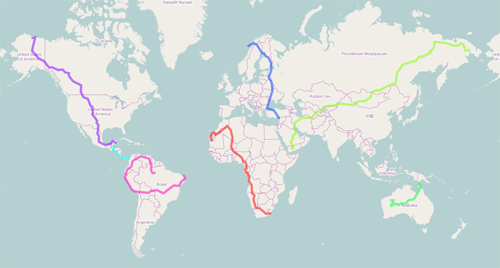
The road network used for the computation was extracted from OpenStreetMap data. This is a fairly big graph: roughly 80 million nodes and 200 million edges. We did not consider ferry connections, and we thus computed the diameter of the largest strongly connected components of the network. Surprisingly enough (for European drivers at least), North and South America are not road-connected. The longest trip in South America circumnavigates the Amazon. The pictures bellow feature some diameter computations on restricted parts of the network (continents and several countries or states).
 |
| Continent longest road trips |
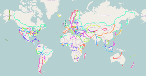 |
| Country longest road trips |
The worst-case complexity of computing the diameter of a graph is conjectured to be quadratic in the size of the graph (more precisely the strong exponential time hypothesis (SETH) implies that diameter cannot be computed in sub-quadratic time). The basic algorithm consists in computing the distance between all pairs of nodes (and it is not known how to do better in general). This impractical for large graphs such as road networks. However, we could rely on efficient heuristics developed partly in Gang (see papers bellow).
We have implemented a variant of the heuristic presented in [2,3] that works
as follows. It consists in performing successive sweeps from selected nodes of
the graph. A sweep from node
This heuristic is particularly efficient when some nodes have sum of excentricities close to the diameter and few nodes are diametral. This is the case in road networks where most strongly connected components require less than 10 sweeps for the diameter computation. However, some parts of the network require more computations. This is the case for Europe that required 146 sweeps. Texas was tough also and required 198 sweeps but Corsica with 107 sweeps for fifteen thousand nodes only was more difficult compared to its size. The regions that required more than 100 sweeps are given in the table bellow. (Note that in general some graphs may require one sweep per node and the heuristic then computes all distances for all pairs of nodes.)
| Most difficult diameter computations | |||
|---|---|---|---|
| Region | Graph size | Diameter length (travel time) | Number of sweeps used |
| Corsica | 14916 | 3h 26mins | 107 |
| Wisconsin | 425765 | 7h 17mins | 110 |
| Third largest Canary island | 22519 | 1h 35mins | 124 |
| Taiwan | 197853 | 6h 24mins | 133 |
| Kansas | 371004 | 8h 51mins | 136 |
| Europe | 24206021 | 2days 12h 49mins | 146 |
| Spain | 2018009 | 12h 8mins | 160 |
| Texas | 2003981 | 14h 13mins | 198 |
We now detail the selection algorithm used as it is a variant of the one presented in [2,3]. It selects any node for the first sweep and then it selects in turn a node with: minimal lower bound of out-excentricity, maximal upper bound of in-excentricity, minimal sum of lower bounds of in- and out-excentricities, maximal upper of bound out-excentricity, minimal lower bound of in-excentricity, maximal sum of upper bounds of in- and out-excentricities. We break ties by prefering nodes with distinct lower and upper bound of excentrity and using the sum of distances to sources of sweeps performed so far.
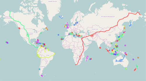
Similar heuristic can also be used to find the radius of the network, that is the minimal out-excentricity of a node in the network. We could compute the centers of all components of the road network, that is nodes with minimal excentricities. As shown on the map bellow, the center of the largest component appears to be in Iran near Turkmenistan border. Any point in Africa, Asia or Europe can be reached within 5 days and 5 hours from that point.
Graphs extracted from GeoFrabrik data in September 2015 (files are in 9th DIMACS format).